Reproducible Reports

With R, Knitr, LaTeX and Markdown

Claas-Thido Pfaff
http://cpfaff.github.io/reproducibility

Download

What is reproducible reporting?

  • Imagine you get an E-Mail

Dear Claas

I was working on an experiment over the last two weeks. Now
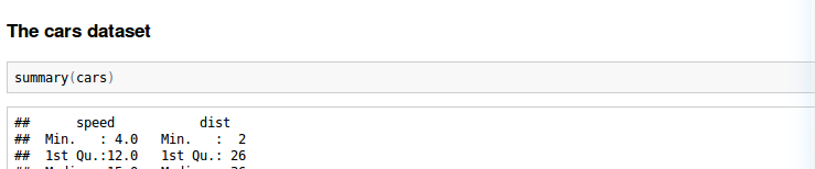
I am currently analysis the data in R and writing down everything
for a report. Could you be so nice and read through my document
and tell me what you think about it so far?
-- All the best Karl

Attachment

  • You are confused

    • only one file?
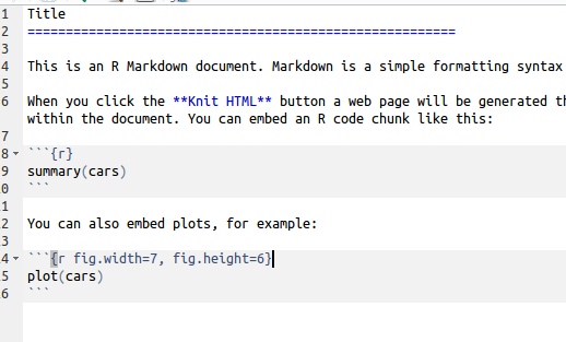
    • which file type (.Rmd) ?
  • But RStudio can open it!

    • you dont understand the syntax! (A mix of text and code?)

What is reproducible reporting?

  • You ask him

Dear Claas

The ending (.Rmd) stands for R-Markdown. Markdown is a
lightweight markup language for text. It can be mixed
with R-Code and then we speak of R-Markdown.

The document can be turned into an nicely formatted HTML page
where the code is executed and replaced by its output. Just install the knitr R package and hit the knit to HTML button in your RStudio!
-- All the best Karl

  • is R-Markdown

    • Textfile with markdown markup + R-Code
    • knitr can somehow turn this to HTML
  • We follow his instructions and install knitr

What is reproducible reporting?

  • R-Studio way: Packages > Install Packages

    deep thought

  • On console:

    • install.packages("knitr")

Get R-Studio

What is reproducible reporting?

  • Knit his file:

    • hit knit HTML button

    • you get HTML output

  • You start to get the idea!

    • only 1 document
    • prevent copy + paste, always up to date
    • saves work time and your nerves, but HTML?

What is reproducible reporting?

  • Knitr R package (Yuhui Xie, 2012)

    • dynamic report generator
  • Markup languages:

  • Markdown -> HTML

    • Knitr: .Rmd -> .md -> .html
    • Generate HTML reports (e.g research blogs, etc)
  • LaTeX -> PDF

    • Knitr: .Rnw -> .tex -> .PDF
    • Generate PDF reports (for Ba./Ma. Thesis, etc.)

Knitr

What is reproducible reporting?

  • Definition:

Reproducible reporting is a techique of research report generation
where we intermix the documentation with the analysis script. We
can turn a source document (e.g .Rmd) into nicely formatted output
documen. This supports the fundamental scientific aim of reproducibility.
Reproducibility means the ability to repeat an entire experiment or study,
either by the original researcher or by someone else working independently
on the same topic. Thus this form of report enables you - or anyone else
with access to that report document to easily reproduce your results.

  • Promotes:
    • Accuracy and correctness
      => others check what we have done!
    • Extensibility and modfiability
      => others can directly build on top of our work!

Read on

R-Markdown and R-Studio

  • Integration:

    • Create a .Rmd file (file > new > R-Markdown)

    • Content sensitive navigation options and syntax help:

R-Markdown Syntax

  • Optional metadata section (embraced by ---)
  • Example:
---
title: "This is my test title"
author: "Claas-Thido Pfaff"
date: "06.09.2014"
output: html_document
---


Markdown Syntax (headers)

  • Headers

    # H1
    ## H2
    ### H3
    ...
    ###### H6
    
    Some text above ....
    
    ### This is a h3 header 
    
    Some text below ...
    

Markdown Syntax (lists)

  • Numbered list (digits)

    1. Element one
    2. Element two
    3. Element three


Markdown Syntax (lists)

  • Bullet list
    • symbols: *, +, -,
    • nesting with 4 spaces
* Element one
* Element two
  - Subelement

Your turn (lists)

  1. Create new .Rmd file (file > new > R-Markdown)
  2. Edit the metadata section and remove the rest
  3. Save the file to desktop
  4. Use it to document upcomming tasks in this course
  5. Create headers H1: "Reproducible Reporting" and H2: "Markdown Lists"
  6. Create a numbered and a bullet list (try nesting)
  7. Knit to HTML
  8. What happens if you use only the number 1 in a list? Why?
1. Element one
1. Element two
1. Element three
  1. Subelement

Your turn (lists)

  • Markdown is turned into HTML
    • Numbered lists look like this:
<ol>
  <li> Element one </li>
  <li> Element two </li>
  <li> Element three </li>
    <ol>
      <li> Subelement </li>
    </ol>
</ol>
  • Same goes for the bullet lists but <ul>
  • This shows content and styling are decoupled in HTML
  • The styling is done via CSS rules!

Markdown Syntax (emphasis)

This is *italic*
  • This is italic
This is **bold**
  • This is bold
This is ***bold and italic***
  • This is bold and italic

  • Example

Markdown Syntax (quotes)

  • Source
> 42 is the answer to the meaning of life, 
> the universe, and everything.
> – *Douglas Adams*
  • Output

42 is the answer to the meaning of life, the universe, and everything.
Douglas Adams

  • Example:


Markdown Syntax (tables)

  • Source (align colon)
| Left align | Right align | Center align |
|:-----------|------------:|:------------:|
| This       |        This |     This     |
| column     |      column |    column    |
| left       |       right |    center    |
  • Output
Left align Right align Center align
This This This
column column column
left right center

Markdown Syntax (links)

  • URL or path

    [link text](url or relative path "Some Text")
    
  • Example

    [GitHub](https://github.com/ "Build software better, together.")
    

    GitHub

  • You can also simply paste in URLs https://github.com/ (see above)

Markdown Syntax (links)

  • Links as References

    • Reference sections/figures/tables
    • Not as sophisticated as Microsoft Word, Open Office, LaTeX
    • But you can use HTML anchors
  • Set anchor

    <!-- set an html anchor -->
    <a name="abcd"></a>
    
  • Set reference in text

    <!-- refer in markdown syntax -->
    [link text](#abcd)
    

Your turn (tables, links, emphasis)

  1. Create H2 header: "Markdown Tables"
  2. Create table
    • Align (left, center, left)
    • highlight the words (bold, italic)
  3. Create a link to http://www.gbif.de/ display the text "gbif"

    Left align Center align Left align
    This is his is This
    right italic bold
    aligned center gbif
  4. Knit to HTML to see the result

Style your markdown

Your turn (tables, links, emphasis)

  • Source
| Left align | Center align | Left align |
|:-----------|:------------:|:-----------|
| This is    |   his is     | This       |
| right      |   *italic*   | **bold**   |
| aligned    |  center      | [gbif](http://www.gbif.de/) |
  • Output
Left align Center align Left align
This is his is This
right italic bold
aligned center gbif

Markdown Syntax (images)

![deep thought](path/to/image/deep_thought.png "Deep Thought")

deep thought

  • No direct control over size (HTML)

<img src="assets/img/deep_thought.png" alt="deep thought" title = "Deep Thought" style="width: 400px;"/>

Image Source

Markdown Syntax (formulas)

  • Not in basic markdown
    • Need external tools (here mathjax)
  • Inline formulas $ ... $
  • Display formulas $$ ... $$ (<div> formula </div>)
$$V_t(S_t) = \max_{x_t \in \chi_t} \left(C(S_t, x_t) + 
            \gamma \sum_{s^{\prime} \in \mathcal{S}}  
            \mathbb{P}(s^{\prime} | S_t^n, x_t)  
            V_{t+1}^{n-1} s^{\prime} \right)$$
$$V_t(S_t) = \max_{x_t \in \chi_t} \left(C(S_t, x_t) + \gamma \sum_{s^{\prime} \in \mathcal{S}} \mathbb{P}(s^{\prime} | S_t^n, x_t) V_{t+1}^{n-1} s^{\prime} \right)$$

Markdown Syntax (code)

  • code blocks (3 Backticks)

    ```
    Text or code goes here
    ```

    myfunction <- function(x,y){
                  z <- x+y;       
                  return(z)     
                } 
    
  • In line code

    In text `code` hightlight
    

R-Markdown Syntax (code chunks)

  • Put your code into:

A code blocks plus (curly braces, r, options)

```{r preparation, cache = TRUE, include = TRUE, echo = TRUE}
x = c(1,2,3,4,5)
y = summary(x)
```
  • Modify how the chunk is treated (chunk options)
    • include = FALSE (to include chunk in output)
    • echo = FALSE (include source code)
    • cache = TRUE (cache chunk)

Knitr chunk options

R-Markdown Syntax (inline code)

Prepare Code:

Option: include = FALSE

```{r preparation, include = F}
x = c(1,2,3,4,5)
mean_of_x = mean(x)
```

Use in your text with inline code chunks:

Lorem ipsum dolor sit ` r x + 10` amet, consetetur sadipscing  
elitr, the mean of x is ` r mean_of_x` ...

Lorem ipsum dolor sit 11, 12, 13, 14, 15 amet, consetetur sadipscing
elitr, the mean of x is 3 ...

R-Markdown Syntax (plots)

  • Options
    • figure.width
    • figure.height
    • fig.align [center, left, right]

Example plot:

```{r how_to_include_plots, fig.width = 8, fig.height = 5, fig.align = 'center'}
require(ggplot2)
qplot(Sepal.Length, Petal.Length, data = iris, color = Species,
          xlab = "Sepal Length", ylab = "Petal Length",
          main = "Sepal vs. Petal Length in Fisher's Iris data")
```
  • The width and height are in inch!

R-Markdown Syntax (plots)

qplot(Sepal.Length, Petal.Length, data = iris, color = Species,
  xlab = "Sepal Length", ylab = "Petal Length",
  main = "Sepal vs. Petal Length in Fisher's Iris data")

plot of chunk unnamed-chunk-4

Your turn (plots)

  1. Create H2 header: e.g "R-Markdown" and H3: e.g "Plots"
  2. Create a chunk that is not displayed! (hint: include)
    • load the ggplot2 package in that chunk
  3. Create another chunk (use qplot)
    • Dataset mtcars
    • x = mpg (miles per US galon)
    • y = wt (weight in lb (pound))
    • if you like map cyl (cylinders) to color
  4. Knit to HTML
  5. Play around with the alignment and size options!
    • center the plot!
    • resize till it looks correct

Your turn (plots)

The preparation chunk:

```{r preparation, include = F}
require(ggplot2)
```

Needs option: include = FALSE

  • If startup messages appear use:
suppressPackageStartupMessages(library(gdata))

Your turn (plots)

The plot chunk:

```{r plotchunk, fig.align = 'center', fig.width = 6, fig.height = 4}
qplot(mpg, wt, data=mtcars, colour=cyl)
```

plot of chunk unnamed-chunk-5

R-Markdown Syntax (tables)

  • Knitr can create markdown tables for you!

needs chunk option: results = 'asis'

```{r results = 'asis'}
kable(head(iris[,1:3]), format = "markdown")   
```
  • kable parameters:
    • align = c("c", "l", "r")
    • digits = 3
    • row.names = T/F

R-Markdown Syntax (tables)

  • Knitr can create markdown tables for you!
    • needs chunk option: results = 'asis'
kable(head(iris[,1:3]), format = "markdown")
Sepal.Length Sepal.Width Petal.Length
5.1 3.5 1.4
4.9 3.0 1.4
4.7 3.2 1.3
4.6 3.1 1.5
5.0 3.6 1.4
5.4 3.9 1.7

Your turn (tables)

  1. Create H3 header: e.g "Automagical Tables"
  2. Create a chunk that is not shown! (hint: include)
    • prepare 7 first rows of the mtcars dataset in a variable (hint: head)
  3. Create another chunk
    • use kable to display the 7 rows (hint: asis)
    • truncate the digits to 1
  4. Knit to HTML

Your turn (tables)

The preparation chunk:

```{r preparation, include = F}
subset_of_mtcars = head(mtcars, 7)
```
  • sets include = F

The table chunk:

```{r themagictable, results = 'asis'}
kable(subset_of_mtcars, format = "markdown", digits = 1)
```
  • as output is markdown results = 'asis'
  • truncate digits = 1

Your turn (tables)

The table:

kable(subset_of_mtcars, format = "markdown", digits = 1)
mpg cyl disp hp drat wt qsec vs am gear carb
Mazda RX4 21.0 6 160 110 3.9 2.6 16.5 0 1 4 4
Mazda RX4 Wag 21.0 6 160 110 3.9 2.9 17.0 0 1 4 4
Datsun 710 22.8 4 108 93 3.8 2.3 18.6 1 1 4 1
Hornet 4 Drive 21.4 6 258 110 3.1 3.2 19.4 1 0 3 1
Hornet Sportabout 18.7 8 360 175 3.1 3.4 17.0 0 0 3 2
Valiant 18.1 6 225 105 2.8 3.5 20.2 1 0 3 1
Duster 360 14.3 8 360 245 3.2 3.6 15.8 0 0 3 4

Your turn (tables GFOE 2014)

  • Create H3 header: e.g "Automagical Tables"
  • Create a chunk that is not shown!
    • load the rbefdata package (require)
    • set the options (cretentials, URL, bef.options)
    • download the datasets (proposal #1)
bef.portal.get.datasets.for_proposal()
  • Create another chunk
    • use kable to display the 7 rows (hint: asis)
  • Knit to HTML

Can I publish markdown?

  • GitHub (Software Development Platform)

    • Version management based on Git
    • Github Pages (used for this presentation!)

    Github My Paper

Can I publish markdown?

  • RStudio and RPubs

    rpubs

  • Howto?

    • Knit: .Rmd -> .md -> .html
    • In preview click publish (needs account!)

    rpubs

Can I publish markdown?

  • No journal accepts markdown! (afaik)
  • Authorea (Online Editor)

    • Harvard University and the Harvard-Smithsonian Center for Astrophysics

    Authorea Homepage

Authorea

Can I publish markdown?

  • But a few accept LaTeX!
  • Authorea (Online Editor)
    • Write in md export to LaTeX

Authorea Export Selection

Where else markdown is used?

Prepare for LaTeX and Knitr

  • Install Latex

    • for PDF report generation
  • MikTeX (Windows)

    • Basic LaTeX-Distribution
  • Install instruction

    • Choose a location to install
    • Preferred paper (A4)
    • Install missing packages (ask me first)
  • Mac users can choose MacTeX

  • Linux users can install TeXlive (package manager)

Prepare for LaTeX and Knitr

  • Integration:

    • Tools > Options > Sweave (Select knitr)

LaTeX and R-Studio

  • Integration:
    • File > new > R Sweave (LaTeX + Noweb)
% preamble
\documentclass{article, report, book, letter}

% load packages here/general layout

% document body
\begin{document}

Some text ...

\end{document}
  • Content sensitive navigation options and syntax help:

LaTeX Syntax

  • Environments

    \begin{environment}
    Some text affected by the environment
    \end{environment}
    
    • like \begin{document} ... \end{document}
  • Commands

    \command{some text} 
    
    • like \textbf{bold face text here}

LaTeX Syntax (title page)

  • Title page

  • Commands (preamble)

    • \title{}
    • \author{}
    • \date{}
% preamble
\title{The Triangulation of Titling Data in
       Non-Linear Gaussian Fashion via $\rho$ Series}
\date{October 31, 475}
\author{John Doe \\ Magic Department, Richard Miles University}
  • In document body use \maketitle

Your turn (title page)

  • Create new R Sweave file in RStudio
    • save file into own folder! (name it e.g mydocumentation.Rnw)
    • if you have \SweaveOpts{...} in there delete it!
  • Not all classes have a title page by default!
    • change to other class e.g to report
    • or modify with options \documentclass[titlepage]{article}
  • Add some example
    • Title
    • Author
    • Date
  • Knit it to PDF

LaTeX Syntax

  • Headers
\part{}
\chapter{} % missing in report
\section{} 
\subsection{}
\subsubsection{}
\paragraph{}
\subparagraph{}
  • Lists (itemize, enumerate, description \item[highlighted] some text)
\begin{itemize}
  \item Element One
  \item Element Two
\end{itemize}

LaTeX Syntax

\textrm{roman text}
\textsf{serif text}
\textbf{bold face text}
\textit{italic text} 
\textsl{slanted text}
\emph{emphasized text}
  • what is the difference between italic/slanted?
  • emph is cool
    • always emphasies no matter where your use it

LaTeX Syntax

  • Code blocks (verbatim)
\begin{verbatim}
def say_hello(name)
   greeting_string = "Hello #{name}"
   return greeting_string
end
\end{verbatim}
  • Preserve line breaks
    • and indent
def say_hello(name)
   greeting_string = "Hello #{name}"
   return greeting_string
end

Do you remember?

Markdown code chunks:

```{r preparation, include = F}
x = c(1,2,3,4,5)
mean_of_x = mean(x)
```

And inline code?

Lorem ipsum dolor sit ` r x + 10` amet, consetetur sadipscing  
elitr, the mean of x is ` r mean_of_x` ...

Same same but different?

  • LaTeX Code chunks
    • syntax different
    • function the same
<<name, key = value>>=
  add your R code here!
@
  • Inline code with
\Sexpr{your r code}

LaTeX Syntax

  • Code chunks example
\section{Results}

<<results, include = F>>=
  a = c(1,2,3,4,5,5)
  b = mean(a)
@
  • And inline code
Lorem ipsum dolor the mean of a is \Sexpr{b} sit amet...
  • NOTE: do not use this to extensively if not necessary!
    • can cluter your source
    • hard to read

LaTeX Syntax

  • figures
\begin{figure}[htbp]
  \centering
    \includegraphics[width=0.5\textwidth]{gull.png}
    \caption{A picture of a gull}
\end{figure}
  • supported formats (pdflatex)
    • jpg
    • png
    • PDF
    • EPS

Your turn (lists, figures)

  • Create section (Reproducible reporting)
  • Create subsection (lists)
  • Create a bullet list and a numbered list (try to nest it)
  • Create subsection (figures)
  • Download the figure (button below)
  • Place it e.g into a figure folder in your document folder
  • Include it
    • center
    • give a caption
  • Knit to PDF
  • resize width parameter (if necessary, Xcm, Xpx, Xin, etc.)

Your turn (lists, figures)

\begin{figure}[htbp]
  \centering
    \includegraphics[width=0.5\textwidth]{figure/deep_thought.png}
    \caption{This is the Deep Thought computer}
\end{figure}
\begin{itemize}
  \item Element One
    \begin{itemize}
      \item Nested Element
    \end{itemize}
  \item Element Two
\end{itemize}

LaTeX Syntax (tables)

  • alignment l,c,r
  • fields separated by &
  • line end \\
\begin{table}[htbp]
  \begin{tabular}{lrc}
    1 & 2 & 3 \\
    4 & 5 & 6 \\
    7 & 8 & 9 \\
  \end{tabular}
\end{table}
  • knitr kable() to the rescue! (try booktabs)
kable(head(iris[,1:3]), format = "latex", booktabs)

Your turn (tables)

  • Create subsection (tables)
  • Create a code chunk not shown in text and prepare
    • from iris dataset (10 rows and column 1 to 4)
  • Create another code chunk
    • use kable to generate a latex table from prepared dataset
  • Knit to PDF
  • include the booktabs package in preamble \usepackage{booktabs}
  • set kable option booktabs = T
  • Knit to PDF
  • Wrap chunk into table environment (hint chunk option echo = F)
    • center \centering
    • give a caption

Your turn (tables)

<<prepare, include = F>>=
  require(knitr)
  iris_prepared = head(iris[,1:4], 10)
@
\begin{table}[htbp]
  \centering
  \caption{Testcaption}
  <<table, results = 'asis', echo = F>>=
  kable(iris_prepared, format = "latex", booktabs = T)
@
\end{table}

LaTeX Syntax

  • Links (URL)
    • reuiqres \usepackage{hyperref}
\url{<my_url>}
\href{<my_url>}{<description>}
  • References: via label <-> reference mechanism
\begin{figure}[htbp]
  \centering
    \includegraphics[width=0.5\textwidth]{gull.png}
    \caption{A picture of a gull}
    \label{fig:mylabel}
\end{figure}

Lorem ipsum dolor sit amet, \ref{fig:mylabel} consetetur sadipscing elitr,

LaTeX Syntax

  • Contents
    • based on sectioning commands
\tableofcontents
  • List of figures
    • based on \captions{}
\listoffigures
  • List of figures
    • based on \captions{}
\listoftables

Your turn (contents)

  • generate a
    • table of contents
    • list of figures
    • list of tables
  • knit to PDF
  • add a new page after the contents if necessary \newpage
  • knit to PDF

Include online repositories!

  • rOpenSci (community, R package development, wrapping science APIs)

  • Packages e.g
    • Dryad (Data publishing service), Mendeley (Citations)
    • taxize (species name resolver), GBif (Species Distribution Data)

Include online repositories!

  • Example from my Open-Science-Paper LaTeX class
\ospFramedEnv*[label = fig:distmap]{
<<distmap_two, fig.width=10, fig.height=5, echo=FALSE, message=FALSE>>=
  osp_distmap(species=c('Accipiter erythronemius', 'Junco hyemalis', 'Aix sponsa'))
@
}{Lorem ipsum dolor sit amet, Brautente, . Aenean
  commodo ligula eget dolor. Aenean massa. Cum sociis natoque penatibus et magnis
  dis parturient montes, nascetur ridiculus mus. Donec quam felis, ultricies nec,
  pellentesque eu, pretium quis, sem.}
  • Own enviroment

\ospFramedEnv*[options]{code chunk}{caption text}

  • Own R function to fetch species data (GBIF)

osp_distmap(species=c('Accipiter erythronemius', 'Junco hyemalis', 'Aix sponsa'))

Include online repositories!

How does this work in detail?

Wrapup: Which format to choose?

  • Markdown

What happens if you ask for too much power from Markdown?
Yihui Xie

Wrapup: Which format to choose?

  • LaTeX
    • designed to create PDF
    • harder to learn and write
    • choose if you need to print it!
    • books e.g LaTeX Companion (Frank Mittelbach, Michael Goossens)
    • good classes available (open-science-thesis, papaper, koma-script)


Reproduce this slides!

  • download the slides (button below!)

  • unzip the archive

  • Open the folder

    • open in Rstudio: index.Rmd
  • Knit it to HTML!

Get this presentation

Reproduce this slides!

  • Install prerequisites
# the devtools package
install.packages("devtools")
require(devtools)
# Install slidify from github
install_github('slidify', 'ramnathv')
install_github('slidifyLibraries', 'ramnathv')
require(slidify)
  • NOTE: Do not write into the file you downloaded!

  • Knit to HTML again

What is reproducible reporting?

  • Open your R-Studio (+ new R script)

  • try:

require(knitr)
require(rmarkdown)
require(ggplot2)
  • Create a folder on your desktop (mylibrary)

  • Add that folder to you library paths in R

.libPaths( c( .libPaths(), "c:/users/username/desktop/mylibrary"))
  • Install the requirements
install.packages(c("knitr", "rmakrdown", "ggplot2"), lib = "c:/users/username/desktop/mylibrary")